A practical guide to SSE SIMD with C++
First published 22. September 2009
This is a guide to Streaming SIMD Extensions with operation system independent C++. Also the details and troubles of SIMD designing with SSE will be addressed in detail.
- 1.0 Introduction
- 2.0 What is SIMD?
- 3.0 Effective use of SSE
- 4.0 Data structures with SSE
- 5.0 Mask operations
- 6.0 C++ SSE header
- Algorithm example 1 - Vector normalization
- Algorithm example 2 - N-particle dynamics
- Algorithm example 3 - Ray sphere intersection
- Algorithm example 4 - Cone quad intersection
- 7.0 Conclusions
- References
- Sources for all algorithms
1.0 Introduction
Current personal computer CPUs have the capability for up to four times faster single precision floating point calculations when utilizing SSE instructions. Unfortunately, the learning curve is high and good documentation on the subject is scarce. In fact, most I could find was endless reference manuals listing available instructions and short tutorials, but little discussion on SSE and generally SIMD design concerns. Exception to this was Intel's optimization reference manual, but it is very low level in nature. The examples are mostly in x86. Additionally, Intel's manual is not in liberty to unbiasedly discuss SSE's weak and strong points as it must help to sell CPUs.
The very first problem with SSE is how access the instructions without resorting to writing x86 assembly. To this end, some C/C++ compilers come with so called SSE intrinsics headers. These provide a set of C functions, which give almost direct access to the vectorized instructions and the needed packaged data types. Unfortunately, coding with the C intrinsics is very inconvenient and results in unreadable code. I present a case here, that this can be solved with C++ operator overloading capabilities without sacrificing performance. Additionally, each version of SSE is accessed by a different intrinsics header and the correct selection and detection should be handled by the wrapping C++ class.
The second problem is that converting algorithms to effectively
use even width four SIMD, as used by SSE, is at most times a very nontrivial task. In fact, depending on the problem domain, not infrequently vectorization is not
worth the trouble versus the possible benefit. However, in some cases it is the
difference between rendering an image 60 frames per second versus 15
frames per second or running a scientific calculation in a week instead of a month.
This guide addresses both of the above mentioned problems. Several algorithms will be transformed into SIMD design and the arising practical difficulties will be discussed. A convenient way to access the SSE extensions with the C++ operator overloading capabilities will be demonstrated. Performance benefits will be determined by benchmarking and evaluating the compiler's instruction output.
2.0 What is SIMD?
SIMD stands for Symmetric Instructions and Multiple Data. The same set of instructions is executed
in parallel to different sets of data. This reduces the amount of hardware
control logic needed by N times for the same amount of calculations, where N is the width of the SIMD unit. SIMD computation model is illustrated in figure 1.
| Figure 1 |

|
The huge downside of SIMD is that the N paths can not be processed differently while in real life algorithms there will be need to process different data differently. This kind of path divergence is handled in SSE either by multiple passes with different masks or by reverting to processing each path in scalar. If large proportion of an algorithm can be run without divergence then SSE can give benefit. Generally, the larger the SIMD width N, the bigger the pain of getting all the speed out of the processing units.
Another illustration of SIMD (copied from Intel) is pictured in figure 2. It underlines the vertical nature of most SSE operations. This concept of data being horizontally for SSE will be utilized through this guide.
| Figure 2 |
 |
SIMD compared to other levels of parallel computing
In
shared memory (thread) level parallelization different parallel paths can execute completely unique set of instructions. This makes for a much simpler parallel programming for example through an API like OpenMP. This is also true for parallelization between
different calculation units without shared memory. However, then usually communication has to be coded in manually through an interface like MPI.
Both of those are MIMD or multiple data and multiple instructions. Note that all of these parallel concepts can and should be utilized at the same time. For example MPI can be used to divide a job between computation units. Then OpenMP used to divide a part of the job between available threads. Finally vectorization can be utilized inside each thread. This is illustrated in figure 3:
| Figure 3 |
 |
3.0 Effective use of SSE
SSE 2.0 up to the currently latest version 4.2 can process four single precision (32-bit) floating point numbers or two double precision (64-bit) floating point numbers in vectorized manner. If this is not enough precision then SSE will be of no use. Furthermore for double precision floating point data there is a realistic potential for speedup of less than 2x to begin with.
Algorithms can be simple unsuitable for SIMD processing. The less single instruction and multiple data parallel parts there are the less speedup there will be. The processing needs to be mostly coherent.
In most cases, only algorithms that are actually expensive enough or run enough times to be significant in total application run time should be vectorized, because of the additional work. Several examples of good or known candidates for vectorization from different fields of science follows:
- Graphics
- Rasterization of triangles, ray tracing of coherent rays, shading pixels with a coherent shader.
- Physics
- N-body dynamics like gravitation between mass points, motion of atoms in potentials or particle dynamics.
- Mathematics
- Matrix operations in general and linear algebra, analytical geometry like intersection tests between primitives
Generally, of course, anything that be done in parallel mostly coherently with the same set of instructions is a candidate.
Data storage and byte boundary alignment
Intel's and AMD's processors will transfer data to and from memory into registers faster if the data is aligned to 16-byte boundaries. While compiler will take care of this alignment when using the basic 128-bit type it means optimally data has to be stored in sets of four 32-bit floating point values in memory. This is one more additional hurdle to deal with when using SSE. If data is not stored in this kind of fashion then more costly unaligned scalar memory moves are needed instead of packaged 128-bit aligned moves.
Intel optimization manual says: "Data must be 16-byte aligned when loading to and storing from the 128-bit XMM registers used by SSE/SSE2/SSE3/SSSE3. This must be done to avoid severe performance penalties."
Long code blocks and register usage
Effective SSE will minimize the amount of moving of data between memory subsystem and the CPU registers. The same is true of scalar code, however, the benefit is higher with SSE. Code blocks should be as long as possible, where the data is loaded into SSE registers only once and then results moved back into memory only once. Storage to memory should be done when data is no longer needed in a code block. What I mean by a code block is a pathway in code that has no boundaries that can no be eliminated by a compiler. An example of a boundary would be a function call that the compiler can not inline.
While the compiler will be of great help for this optimization by inlining functions, algorithms and program structure have to be designed with this in mind. SSE versions between 2.0 to 4.2 have total of eight 128-bit registers available in 32-bit mode and sixteen in 64-bit mode. The latter can hold total of 64 single precision floating point values in registers.
4.0 Data structures with SSE
The basic SSE 32-bit floating point data
type is four floating point values in what is usually considered a horizontal structure:

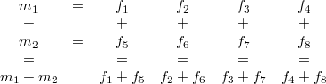
It is horizontal because most SSE instructions operate on data vertically. Note that this is a 128-bit continuous block of four 32-bit floats in memory. In code this will be called vec4. For example a vertical sum between m1 and m2 can then be illustrated like this:
How
should data be then arranged into these 4xhorizontal structures? It depends on the application. Let's
say the data is a set of three dimensional vectors. These could be
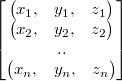
normally arranged into array of structures (AOS) like this:
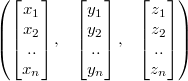
or in structure of arrays (SOA) like:
For SSE these structures should be altered to incorporate the horizontal block of four floats. The first (AOS) looks then like (notice the commas):
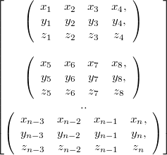
Notice how for each element in structure "x" was just replaced with "x1 x2 x3 x4" and the same for y and z. Similarly the latter (SOA):
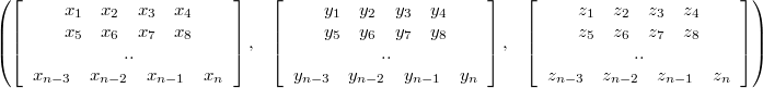
Especially useful basic type is the 4x3 matrix like block in the first (AOS):
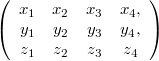
Note that it is a struct with three elements:
It can also be obtained from SOA format just as easily by taking the nth elements from each array. The difference between the two then is that depending on the task the other uses memory cache more efficiently.
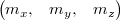
This block of four three dimensional vectors will be called mat4x3 data type in the code. To see its usefulness we will normalize these four vectors in it. To
achieve that first 3 multiplications followed by 3 additions are needed
vertically as follows:
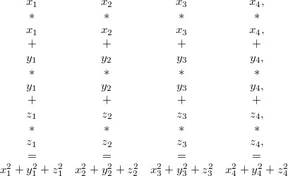
Continuing
from that we can execute a special SSE square root instruction to the
result and multiple each three of the original components with its reciprocal to
get the final result (also mat4x3, of course):
This normalization can be seen in the first code example.
5.0 Mask operations
With width four SIMD at least four bits are needed to represent a mask:

SSE uses the same 128-bit type for representing masks returned by floating point comparisons. Single float's byte sequence 0x00000000 in hexadecimals represents false and 0xFFFFFFFF represents true. SSE has comparison instructions for all the basic arithmetic comparisons like greater or equal than.
Mask are then produced by using standard C++ comparison operators between two vec4 types:
or listing all the elements:

The resulting mask can then be used to conditionally only write to parts of vec4 or deciding a path based on whether all the bits are set, none of them are set, or some of them are set.
Examples of different kinds of control logic turned into mask operations can be found in the algorithm examples.
6.0 C++ SSE header
In February 2009 Krzysztof Jakubowski posted a full implementation of C++ wrapping over the 32-bit floating point and the 32-bit integer SSE C intrinsics on a ray tracing Internet forum called ompf. It is called veclib and it s licensed with very permissive zlib license. From my experiments with that implementation this guide was born.
Generally, when writing vector code in vector notation in C++, one can in my experience do so without any overhead to worry about by using expression templates. Basically expression templates help avoid unnecessary temporaries over naive C++ operator overloaded implementations. An implementation of this is a BSD-type licensed piece of code called cvalarray.
What I advocate is to use these two implementations together to get, as far as I know, the fastest and neatest freely available C++ implementation of basic 3D vectors and SSE types. Of course, for some specific higher level tasks there are better options, like Eigen for linear algebra. To get better notation compared to what veclib uses I took example of GLSL specifications to come up with this for writing SSE code:
| C++ vector types with SSE for single precision (32-bit) |
vec2,vec3,vec4 floating point vector vec2b,vec3b,vec4b mask type for floating point vector ivec2,ivec3,ivec4 signed integer vector ivec2b,ivec3b,ivec4b mask type for signed integer vector mat4x2,mat4x3,mat4x4 4 column floating point matrix (SSE) |
Also any of these can be prefixed with "p" for double precision. And this is then a full header file, that implements part of these types:
#include "cvalarray.hpp"
#include "veclib.h"

typedef veclib::f32x4 vec4;
typedef veclib::f32x4b vec4b;
typedef veclib::i32x4 ivec4;
typedef veclib::i32x4b ivec4b;
typedef n_std::cvalarray<vec4,2> mat4x2;
typedef n_std::cvalarray<vec4,3> mat4x3;
typedef n_std::cvalarray<vec4,4> mat4x4;
typedef n_std::cvalarray<float,2> vec2;
typedef n_std::cvalarray<float,3> vec3;
typedef n_std::cvalarray<double,2> pvec2;
typedef n_std::cvalarray<double,3> pvec3;
The idea here is that each of these has the exact same user interface. Brackets [] are used for element access and arithmetic with operators works as it should. Easy to remember.
Veclib
Documentation of the veclib's interface can be found at veclib.h. For how the library can and should be used refer to the algorithm examples.
Strengths / weaknesses of this approach
Code is easy to read and to type. The conversion from scalar to vectorized form or the other way around can be at best copy paste with little modifications.
Proven real world viability and efficiency by this very guide.
Code is not tied to any particular low level implementation including even the intrinsics or veclib. A few special functions, like a vectorized square root and a conditional move, do not, however, satisfy this criteria.
The biggest weakness is the lack of implementations of packaged version of basic mathematical functions not provided by SSE instructions at hardware level. These include the trigonometric functions, the exponential function and basically everything except basic arithmetic and a square root. Free implementations of some of these on top of the intrinsics are available online. Maybe AMD's open source SSEPlus project could be of service here. Intel's commercial Math Kernel Library has many implemented.One has to be very careful when coding on this high level to not do just anything that is possible. It can still give correct output, but potentially degrade or kill performance. What are behind the C++ operators are the C intrinsics functions and SSE types, and a compiler doesn't produce optimal code for all usages. The algorithm examples in this guide help document the possible severity of this problem and help to learn how to avoid it.
Veclib selects the correct implementations of the high level operations based on the version of SSE selected by compiler parameters. For GCC this is done with "-msseX" where X is the version or "-march=native" for the best supported version. However, this means a single binary will support only the selected version of SSE. Optimally it would be desirable to have a single binary perform run time selection of the SSE path based on the detected CPU. Maybe several binaries compiled for the different versions of SSE could be combined with CPU detection to have such support for an application.
Veclib is unlikely to see much development in the future as the author (Krzysztof Jakubowski) has stated he has discontinued his project that included veclib. This means a question mark for support of the current SSE4 extensions or the upcoming AVX. However, SSE3/SSSE3/SSE4 provided little extra for most usages of floating point over SSE2. Also veclib is also just a thin wrapping over the intrinsics to begin with and so easy to modify. Furthermore Intel states in May 2008 AVX document: "Most apps written with intrinsics need only recompile".
Algorithm example 1 - Vector normalization
As noted in the chapter about data structures, vector normalization can be implemented with SSE in a very straightforward manner:
// Example one. Normalizing AOS vectors

// Scalar
inline void normalize(std::vector<vec3>& data)
{
  for (int i=0;i<data.size();i++)
  {
    vec3& m = data[i];
    m /= sqrtf( m[0]*m[0] + m[1]*m[1] + m[2]*m[2] );
  }
}

// SSE
inline void normalize(std::vector<mat4x3>& data)
{
  for (int i=0;i<data.size();i++)
  {
    vec4 mx = data[i][0];
    vec4 my = data[i][1];
    vec4 mz = data[i][2];

    vec4 multiplier = 1.0f/Sqrt(mx*mx + my*my + mz*mz);
    mx*=multiplier;
    my*=multiplier;
    mz*=multiplier;

    data[i][0]=mx;
    data[i][1]=my;
    data[i][2]=mz;
  }
}
In the scalar version the explicit loading and unloading of data to and from memory to temporary variables could be avoided notationally by using a vec3 reference. However, in the SSE version vec4 temporary types must be used in order to make compiler produce optimal code. In practice these temporaries will be XMM registers in the assembly code produced. Note that using the mat4x3 type as a reference this could be written in the SSE version as:
// SSE (wrong, mat4x3 elements referenced multiple times)
inline void normalize(std::vector<mat4x3>& data)
{
  for (int i=0;i<data.size();i++)
  {
    mat4x3& m = data[i];
    m /= Sqrt(m[0]*m[0] + m[1]*m[1] + m[2]*m[2]);
  }
}
However, compiler doesn't produce optimal instructions this way. It is able to do so with the scalar version I believe because of the C++ expression templates behind cvalarray implementation of vec3.
Taking a look at what kind of instructions GCC 4.4.2 produces for these here is first the scalar version:
        movss   (%rax), %xmm3
        movss   4(%rax), %xmm2
        movss   8(%rax), %xmm1
        movaps  %xmm2, %xmm0
        movaps  %xmm3, %xmm4
        mulss   %xmm2, %xmm0
        mulss   %xmm3, %xmm4
        addss   %xmm4, %xmm0
        movaps  %xmm1, %xmm4
        mulss   %xmm1, %xmm4
        addss   %xmm4, %xmm0
        movaps  %xmm5, %xmm4
        sqrtss  %xmm0, %xmm0
        divss   %xmm0, %xmm4
        movaps  %xmm4, %xmm0
        mulss   %xmm4, %xmm3
        mulss   %xmm4, %xmm2
        movss   %xmm3, (%rax)
        movss   %xmm2, 4(%rax)
        mulss   %xmm1, %xmm0
        movss   %xmm0, 8(%rax)
And here the SSE:
        movaps  (%rax), %xmm3
        movaps  16(%rax), %xmm2
        movaps  32(%rax), %xmm1
        movaps  %xmm2, %xmm5
        movaps  %xmm3, %xmm0
        mulps   %xmm2, %xmm5
        mulps   %xmm3, %xmm0
        movaps  %xmm1, %xmm4
        addps   %xmm5, %xmm0
        mulps   %xmm1, %xmm4
        addps   %xmm4, %xmm0
        movaps  %xmm6, %xmm4
        sqrtps  %xmm0, %xmm0
        divps   %xmm0, %xmm4
        movaps  %xmm4, %xmm0
        mulps   %xmm4, %xmm3
        mulps   %xmm4, %xmm2
        mulps   %xmm1, %xmm0
        movaps  %xmm3, (%rax)
        movaps  %xmm2, 16(%rax)
        movaps  %xmm0, 32(%rax)
One can notice definitive symmetry between the two even if one understands little to no x86. There are only aligned 128-bit moves in the SSE version and it is almost identical to the scalar version except for packaged instructions instead of scalar, which is a sign of proper code generation by the compiler.
It is worth the effort to go through either version instruction by instruction to be able to understand if the instruction output makes sense or not. This helps with debugging SSE applications tremendously. Definitions of each instruction can be found by a web search.
It is very educational to also look at the "wrong" version:
        movaps  32(%rax), %xmm1
        movaps  16(%rax), %xmm2
        movaps  (%rax), %xmm3
        movaps  %xmm1, %xmm4
        movaps  %xmm2, %xmm5
        mulps   %xmm1, %xmm4
        mulps   %xmm2, %xmm5
        movaps  %xmm3, %xmm0
        mulps   %xmm3, %xmm0
        addps   %xmm5, %xmm0
        addps   %xmm4, %xmm0
        sqrtps  %xmm0, %xmm0
        divps   %xmm0, %xmm3
        divps   %xmm0, %xmm2
        movaps  %xmm3, (%rax)
        movaps  %xmm2, 16(%rax)
        divps   %xmm0, %xmm1
        movaps  %xmm1, 32(%rax)
In this case there is actually nothing wrong with it, except it does what was asked: It performs three divisions instead of three multiplications in the end, which slows it down. Replacing /= with *= and adding 1.0f/ results in yet another version:
        movaps  (%rax), %xmm3
        movaps  32(%rax), %xmm1
        movaps  16(%rax), %xmm2
        mulps   %xmm1, %xmm1
        movaps  %xmm3, %xmm0
        mulps   %xmm2, %xmm2
        mulps   %xmm3, %xmm0
        addps   %xmm2, %xmm0
        addps   %xmm1, %xmm0
        movaps  %xmm4, %xmm1
        sqrtps  %xmm0, %xmm0
        divps   %xmm0, %xmm1
        movaps  %xmm1, %xmm0
        mulps   %xmm1, %xmm3
        mulps   32(%rax), %xmm0
        mulps   16(%rax), %xmm1
        movaps  %xmm3, (%rax)
        movaps  %xmm1, 16(%rax)
        movaps  %xmm0, 32(%rax)
The problem with this one is that it once again does what was asked: It performs the multiplication "mulps 32(%rax), %xmm0" not with purely XMM registers. These two cases should help to illustrate why it is unfortunately necessary to explicitly tell the compiler what to do when dealing with vec4 types. Problems can be usually avoided by not using the mat4x3 type as a reference or worst as a temporary. It should only be used for loading and extracting data at the start and end of a function or more optimally the longest possible code block.
It is also of interest to look at the speed gains from SSE from this implementation. The test hardware is Intel Core 2 Duo E6400. Operating system is 64-bit Linux and the compiler is GCC 4.4.2.

The points are sample means and the standard error tells how the samples were spread. If the functions are forced not to be inlined then the > 4x behavior for N < 10000 disappears. Here we can see a speedup of very close to 4x for normalizing a set of about 20000 vectors. At very large amounts the speedup settles to about 3.4x. As for the reason of the general shape of the curve, anyone is welcome to make a guess. The output between SSE and scalar paths is identical bit to bit.
If normalizing the same data of vectors over and over multiple times the speedup from SSE was about 2.7x-2.2x when number of repetitions is large. The larger speedup applies to data sets smaller than about 20000 and the smaller for larger data sets. This is I believe because the data was moved between memory and registers between each normalization and for some reason this penalizes the SSE implementation more.
Algorithm example 2 - N-particle dynamics
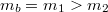
N particles where each particle interacts with all the other particles through a force and the motion is solved by numerical integration. In scalar code this can be effectively solved by defining a Particle class as follows and then executing the force member function once to each pair of particles:
class Particle {
public:
vec3 pos;
vec3 vel;
vec3 acc;
float mass;

Particle(vec3 pos, vec3 vel, float mass)
{
Particle::pos=pos;
Particle::vel=vel;
Particle::acc=0.0f;
Particle::mass=mass;
}

/** Newton's gravitation law */
void force(Particle& p)
{
vec3 diff = pos - p.pos;
float r2=sum(diff*diff);
diff /= sqrt(r2)*(r2+1.0f);
acc   -= diff*p.mass;
p.acc += diff*mass;
}
};
Forces between all the particles can then be solved and a very basic numerical integration implemented as follows:
std::vector<Particle> data1;

// Iterate the following code in a loop
for (int i=0;i<data1.size();i++)
  data1[i].acc=0.0f;

for (int i=0;i<data1.size();i++)
  for (int j=i+1;j<data1.size();j++)
    data1[i].force(data1[j]);

for (int i=0;i<data1.size();i++)
{
  data1[i].vel += data1[i].acc*dt;
  data1[i].pos += data1[i].vel*dt;
}
To transform this into SIMD concept by taking note of SSE alignment requirements we can think as follows: Store four particles in a single structure so that everything that is done for a single particle can be done in parallel to four particles. However, calculating the forces between all the particles isn't anymore as straightforward as force has to be calculated between all particles and not just between particles of different packets. The solution is to calculate the forces to each individual particle from all other packets and additionally from particles in the same packet. The following is an implementation of this concept:
class Particle4 {
public:
mat4x3 pos;
mat4x3 vel;
mat4x3 acc;
vec4 mass;

Particle4(mat4x3 pos, mat4x3 vel, vec4 mass)
{
Particle4::pos=pos;
Particle4::vel=vel;
Particle4::acc=0.0f;
Particle4::mass=mass;
}

/// Calculate forces to each member Particle from another Particle4
void force(Particle4& p)
{
for (int n=0;n<4;n++)
        {
        vec4 diffx = vec4(pos[0][n]) - p.pos[0];
        vec4 diffy = vec4(pos[1][n]) - p.pos[1];
        vec4 diffz = vec4(pos[2][n]) - p.pos[2];
        vec4 r2 = diffx*diffx + diffy*diffy + diffz*diffz;
        vec4 rlen = 1.0f/(Sqrt(r2)*(r2+1.0f));
        diffx *= rlen;
        diffy *= rlen;
        diffz *= rlen;
        acc[0][n] -= sum(diffx*p.mass);
        acc[1][n] -= sum(diffy*p.mass);
        acc[2][n] -= sum(diffz*p.mass);
        p.acc[0] += diffx*mass;
        p.acc[1] += diffy*mass;
        p.acc[2] += diffz*mass;
        }
}

/// Calculate forces between particles inside this Particle4
void insideforces(void)
{
for (int n=0;n<4;n++)
        for (int k=n+1;k<4;k++)
        {
        vec3 diff;
        diff[0] = pos[0][n] - pos[0][k];
        diff[1] = pos[1][n] - pos[1][k];
        diff[2] = pos[2][n] - pos[2][k];
        float r2=sum(diff*diff);
        diff /= sqrt(r2)*(r2+1.0f);
        acc[0][n] -= diff[0]*mass[k];
        acc[1][n] -= diff[1]*mass[k];
        acc[2][n] -= diff[2]*mass[k];
        acc[0][k] += diff[0]*mass[n];
        acc[1][k] += diff[1]*mass[n];
        acc[2][k] += diff[2]*mass[n];
        }
}

};
And solving the motions is implemented then by:
std::vector<Particle4> data2;

// Repeat for number of iterations
for (int i=0;i<data2.size();i++)
  data2[i].acc=0.0f;

for (int i=0;i<data2.size();i++)
{
  data2[i].insideforces();
  for (int j=i+1;j<data2.size();j++)
    data2[i].force(data2[j]);
}

for (int i=0;i<data2.size();i++)
{
  data2[i].vel += data2[i].acc*dt4;
  data2[i].pos += data2[i].vel*dt4;
}
Note that everything except calculation of the forces inside a Particle packet could be vectorized. The speedup from this implementation was at best close to exactly 2x. Not quite satisfactory. In this implementation the forces are calculated from each N packets to the first, second, third and fourth particle inside Particle4 in turn. However, calculating forces to the first particle from all the other packets and then repeating for the three more particles, it is possible to get rid the horizontal sums "sum(diffx*p.mass)" and scalar extracts "vec4(pos[0][n])" from the Particle4 force function. The implementation is modified then as follows:
// Replacement force function for NParticle
void force(NParticle& p, const vec4& posx, const vec4& posy, const vec4& posz, vec4& accx, vec4& accy, vec4& accz)
{
        vec4 diffx = posx - p.pos[0];
        vec4 diffy = posy - p.pos[1];
        vec4 diffz = posz - p.pos[2];
        vec4 r2 = diffx*diffx + diffy*diffy + diffz*diffz;
        vec4 rlen = 1.0f/(Sqrt(r2)*(r2+1.0f));
        diffx *= rlen;
        diffy *= rlen;
        diffz *= rlen;
        accx -= diffx*p.mass;
        accy -= diffy*p.mass;
        accz -= diffz*p.mass;
        p.acc[0] += diffx*mass;
        p.acc[1] += diffy*mass;
        p.acc[2] += diffz*mass;
}
and force calculation:
// Replacement for force calculations
        for (int i=0;i<data2.size();i++)
                {
                data2[i].insideforces();

                for (int n=0;n<4;n++)
                {
                        vec4 posx = data2[i].pos[0][n];
                        vec4 posy = data2[i].pos[1][n];
                        vec4 posz = data2[i].pos[2][n];
                        vec4 accx=0.0f;
                        vec4 accy=0.0f;
                        vec4 accz=0.0f;
                        for (int j=i+1;j<data2.size();j++)
                                data2[i].force(data2[j],posx,posy,posz,accx,accy,accz);
                        data2[i].acc[0][n] += sum(accx);
                        data2[i].acc[1][n] += sum(accy);
                        data2[i].acc[2][n] += sum(accz);
                }
                }
This implementation is much faster. The speed gain is represented in the following figure:

The output was not generally bit wise identical because floating point operations are carried out in different order between the paths. However, calculation precision in both paths is the same. One more additional note is that using the SSE3 haddps inctruction for the horizontal sum made barely any difference to using SSE2 style horizontal sum.
Algorithm example 3 - Ray sphere intersection
Intersection test between a ray and a sphere will be an example of algebraic geometry. Inserting a general line equation:
Into sphere surface equation:
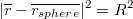
Gives a quadratic equation for t in terms of the known input vectors and R. In code the solution for t can be implemented as follows:
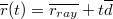
inline bool intersect(const vec3& raydir, const vec3& rayorig,const vec3& pos,
const float& rad, vec3& hitpoint,float& distance, vec3& normal)
{
float a = sum(raydir*raydir);
float b = sum(raydir * (2.0f * ( rayorig - pos)));
float c = sum(pos*pos) + sum(rayorig*rayorig) -2.0f*sum(rayorig*pos) - rad*rad;
float D = b*b + (-4.0f)*a*c;

// If ray can not intersect then stop
if (D < 0)
        return false;
D=sqrtf(D);

// Ray can intersect the sphere, solve the closer hitpoint
float t = (-0.5f)*(b+D)/a;
if (t > 0.0f)
        {
        distance=sqrtf(a)*t;
        hitpoint=rayorig + t*raydir;
        normal=(hitpoint - pos) / rad;
        }
else
        return false;
return true;
This can be vectorized for example by intersecting a packet of four rays against a single sphere. The other possibility is to intersect a single ray against four spheres. There is control logic in the code, which has to be replaced by mask operations. Additionally the vectorized intersection function will be taking a mask, which determines which rays should be touched by the function in the first place. An implementation follows:
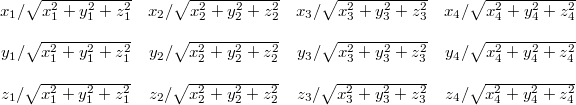
inline vec4b intersect(const mat4x3& raydir, const mat4x3& rayorig, const vec3& pos,
const float& rad, mat4x3& hitpoint, vec4& distance, mat4x3& normal, vec4b& mask)
{
vec4 raydirx = raydir[0];
vec4 raydiry = raydir[1];
vec4 raydirz = raydir[2];
vec4 a = raydirx*raydirx + raydiry*raydiry + raydirz*raydirz;
vec4 rayorigx = rayorig[0];
vec4 rayorigy = rayorig[1];
vec4 rayorigz = rayorig[2];
vec4 b = raydirx * 2.0f * (rayorigx - pos[0]) +
raydiry * 2.0f * (rayorigy - pos[1]) + raydirz * 2.0f * (rayorigz - pos[2]);
vec4 c = sum(pos*pos) + rayorigx*rayorigx + rayorigy*rayorigy + rayorigz*rayorigz -
2.0f*(rayorigx*pos[0] + rayorigy*pos[1] + rayorigz*pos[2]) - rad*rad;

vec4 D = b*b + (-4.0f)*a*c;

mask = mask && D > 0.0f;
if (ForWhich(mask) == 0)
	return mask;

D = Sqrt(D);

vec4 t = (-0.5f)*(b+D)/a;

mask = mask && t > 0.0f;
int bitmask = ForWhich(mask);

// All rays hit
if (bitmask == 15)
	{
	distance = Sqrt(a) * t;
	vec4 hitpointx = rayorigx + t*raydirx;
	vec4 hitpointy = rayorigy + t*raydiry;
	vec4 hitpointz = rayorigz + t*raydirz;
	normal[0]=(hitpointx - pos[0]) / rad;
	normal[1]=(hitpointy - pos[1]) / rad;
	normal[2]=(hitpointz - pos[2]) / rad;
	hitpoint[0]=hitpointx;
	hitpoint[1]=hitpointy;
	hitpoint[2]=hitpointz;
	}
else if (bitmask == 0)
	return mask;
else // some rays hit
	{
	distance = Condition(mask, Sqrt(a) * t, distance);
        vec4 hitpointx = rayorigx + t*raydirx;
        vec4 hitpointy = rayorigy + t*raydiry;
        vec4 hitpointz = rayorigz + t*raydirz;
	normal[0]=Condition(mask, hitpointx - pos[0], normal[0]);
	normal[1]=Condition(mask, hitpointy - pos[1], normal[1]);
	normal[2]=Condition(mask, hitpointz - pos[2], normal[2]);
	hitpoint[0]=Condition(mask, hitpointx, hitpoint[0]);
	hitpoint[1]=Condition(mask, hitpointy, hitpoint[1]);
	hitpoint[2]=Condition(mask, hitpointz, hitpoint[2]);
	}
return mask;
}
Note how the last part of the code had to be divided into three sections, one for when all rays hit, one where part of them hit and one where none of them hit. The Condition and ForWhich functions are part of Veclib and documented by it.
For this algorithm I was unable to get a speedup approaching 4x when all rays were coherent and hit. The vectorized algorithm looks fine as does the machine code output. A figure of the speedup behavior follows:

Algorithm example 4 - Cone quad intersection
A cone is a geometrical shape similar to the waffle under ice cream and a quad is a surface polygon defined by four points in three dimensions. Parallelism inside an ordinary cone quad intersection will be utilized instead of intersecting cone against four quads or four cones against quad. This has the advantage, that nothing outside of the function has to be changed and the disadvantage, that not all parts of the algorithm can be vectorized.
To intersect a cone against a quad three things have to be checked: First whether any of the quad's vertices are inside the cone. Secondly whether any edge of the quad intersects the cone. Thirdly whether the axis of the cone intersects the quad. These can be done in arbitrary order and the order should be selected on the basis of probability for a test to succeed in an application.
Implementation here is based on "Intersection of a Triangle and a Cone by David Eberly", a copy of which is distributed with the source package. The SSE version was implemented before the scalar version:
//	D = cone direction
//	L = cone starting position
//	cphi2 = cosine power 2 of cone angle
//	P = Quad vertices
//
noinline bool ConeQuadIntersection(const vec3& D, const vec3& L, const float& cphi2, mat4x3& P)
{
vec4 LP0 = P[0] - L[0];
vec4 LP1 = P[1] - L[1];
vec4 LP2 = P[2] - L[2];
vec4 LPLP = LP0*LP0 + LP1*LP1 + LP2*LP2;
vec4 cLPLP = cphi2*LPLP;
vec4 LP0D = LP0*D[0] + LP1*D[1] + LP2*D[2];
vec4 LP0D2= LP0D*LP0D;

// check if any vertex is inside cone
vec4b conesidemask = LP0D >= 0.0f;
if (ForAny(conesidemask))
	{
	vec4b insidemask = LP0D2 >= cLPLP;

	if (ForAny(insidemask && conesidemask)) // any point inside?
		return true;
	}
else
	return false; // all on other side of the plane

// Check if any edge intersects cone
vec4 E0,E1,E2; // Edge vectors
E0[0] = P[0][1] - P[0][0];
E0[1] = P[0][2] - P[0][1];
E0[2] = P[0][3] - P[0][2];
E0[3] = P[0][0] - P[0][3];

E1[0] = P[1][1] - P[1][0];
E1[1] = P[1][2] - P[1][1];
E1[2] = P[1][3] - P[1][2];
E1[3] = P[1][0] - P[1][3];

E2[0] = P[2][1] - P[2][0];
E2[1] = P[2][2] - P[2][1];
E2[2] = P[2][3] - P[2][2];
E2[3] = P[2][0] - P[2][3];

vec4 DE = D[0]*E0 + D[1]*E1 + D[2]*E2;
vec4 c0 = LP0D2 - cLPLP;
vec4 c1 = DE * LP0D - cphi2 * (E0*LP0 + E1*LP1 + E2*LP2 );
vec4 Elen2 = E0*E0 + E1*E1 + E2*E2;
vec4 c2 = DE*DE - cphi2 * Elen2;

vec4b mask = c2 < 0.0f && c1*c1 >= c0*c2;

if (ForAny(mask)) // some edge can intersect
	{
	if (ForAll(conesidemask)) // all on the cone side
		{
		vec4b mask2 = mask && 0.0f <= c1 && c1 <= (-1.0f*c2);
		if (ForAny(mask2)) // edge intersects
			return true;
		}
	else
		{
		// unimplemented
		}
	}

// Check if cone axis intersects the quad
vec3 hitpoint;
vec3 planepoint;
planepoint[0]=P[0][0];
planepoint[1]=P[1][0];
planepoint[2]=P[2][0];
vec3 planenormal;
planenormal[0]=E1[0]*E2[1]-E1[1]*E2[0];
planenormal[1]=-E0[0]*E2[1]+E0[1]*E2[0];
planenormal[2]=E0[0]*E1[1]-E0[1]*E1[0];
float length = 1.0f/sqrtf(planenormal[0]*planenormal[0] + planenormal[1]*planenormal[1] + planenormal[2]*planenormal[2]);
planenormal *= length;

if (!RayPlaneIntersection(L, D, planenormal, planepoint, hitpoint))
	return false;

vec3 point = hitpoint - planepoint;

float p1 = ( point[0] * E0[0] + point[1] * E1[0] + point[2] * E2[0] ) / Elen2[0];
float p2 = ( point[0] * E0[1] + point[1] * E1[1] + point[2] * E2[1] ) / Elen2[1];

if (p1 >= 0.0f && p1 <= 1.0f && p2 >= 0.0f && p2 <= 1.0f) // cone inside quad?
	return true;
else
	return false;
}
Basically the first part (vertices inside cone) is vectorized, the second part (edges intersect cone) is vectorized and the last part (cone axis intersects quad) is not. The parallelism comes from there being four vertices and four edges to check in identical way. However an optimal implementation is little different between the scalar and vectorized version. The optimal vectorized version was perhaps even easier to code than the scalar one, because it is very straightforward. In the scalar version if the first vertex or edge test succeeds then the function can immediately return, which lowers the benefit from the vectorized version. The optimal edges to test are also different between the two.
// define scalar versions of vec4 and mat4x3
typedef n_std::cvalarray<n_std::cvalarray<float,4>,3> smat4x3;
typedef n_std::cvalarray<float,4> svec4;
typedef n_std::cvalarray<bool,4> svec4b;

bool ConeQuadIntersection(const vec3& dir, const vec3& pos, const float cosphi2, const smat4x3& P)
{
svec4 pospx,pospy,pospz;
svec4 pospdir;
svec4 posp2;
svec4 pospdir2;

bool anyin=false;
svec4b otherside;

// Check if any of the points in inside the cone
for (int i=0;i<4;i++)
	{
	pospx[i]=P[0][i] - pos[0];
	pospy[i]=P[1][i] - pos[1];
	pospz[i]=P[2][i] - pos[2];
	pospdir[i] = pospx[i] * dir[0] + pospy[i] * dir[1] + pospz[i] * dir[2];

	if (pospdir[i] > 0)
		{
		anyin=true;
		otherside[i]=false;
		posp2[i] = pospx[i]*pospx[i] + pospy[i]*pospy[i] + pospz[i]*pospz[i];
		pospdir2[i] = pospdir[i]*pospdir[i];
		if (pospdir2[i] >= cosphi2 * posp2[i])
			return true;
		}
	else
		otherside[i]=true;
	}

// all on other side of cone
if (!anyin)
	return false;

// Next test edges of the quad for intersection

vec3 edge1;
edge1[0] = P[0][1] - P[0][0];
edge1[1] = P[1][1] - P[1][0];
edge1[2] = P[2][1] - P[2][0];
float edge1l2 = edge1[0]*edge1[0] + edge1[1]*edge1[1] + edge1[2]*edge1[2];

if (!otherside[0] && !otherside[1])
	{
	float diredge = dir[0]*edge1[0] + dir[1]*edge1[1] + dir[2]*edge1[2];
	float c0 = pospdir2[0] - cosphi2*posp2[0];
	float c1 = diredge * pospdir[0] - cosphi2 * (edge1[0]*pospx[0] + edge1[1]*pospy[0] + edge1[2]*pospz[0]);
	float c2 = diredge*diredge - cosphi2 * edge1l2;

	if (c2 < 0.0f && 0.0f <= c1 && c1 <= (-1.0f)*c2 && c1*c1 >= c0*c2)
		return true;
	}

vec3 edge2;
edge2[0] = P[0][2] - P[0][0];
edge2[1] = P[1][2] - P[1][0];
edge2[2] = P[2][2] - P[2][0];
float edge2l2 = edge2[0]*edge2[0] + edge2[1]*edge2[1] + edge2[2]*edge2[2];

if (!otherside[0] && !otherside[2])
        {
        float diredge = dir[0]*edge2[0] + dir[1]*edge2[1] + dir[2]*edge2[2];
        float c0 = pospdir2[0] - cosphi2*posp2[0];
        float c1 = diredge * pospdir[0] - cosphi2 * (edge2[0]*pospx[0] + edge2[1]*pospy[0] + edge2[2]*pospz[0]);
        float c2 = diredge*diredge - cosphi2 * edge2l2;

        if (c2 < 0.0f && 0.0f <= c1 && c1 <= (-1.0f)*c2 && c1*c1 >= c0*c2;
                return true;
        }

for (int i=1;i<=2;i++)
{
if (!otherside[3] && !otherside[i])
        {
        vec3 edge;
        edge[0] = P[0][i] - P[0][3];
        edge[1] = P[1][i] - P[1][3];
        edge[2] = P[2][i] - P[2][3];
        float diredge = dir[0]*edge[0] + dir[1]*edge[1] + dir[2]*edge[2];
        float c0 = pospdir2[3] - cosphi2*posp2[3];
        float c1 = diredge * pospdir[3] - cosphi2 * (edge[0]*pospx[3] + edge[1]*pospy[3] + edge[2]*pospz[3]);
        float c2 = diredge*diredge - cosphi2 * (edge[0]*edge[0] + edge[1]*edge[1] + edge[2]*edge[2]);

        if (c2 < 0.0f && 0.0f <= c1 && c1 <= (-1.0f)*c2 && c1*c1 >= c0*c2)
                return true;
        }
}

// Next check if cone axis intersects quad

vec3 hitpoint;
vec3 planepoint;
planepoint[0]=P[0][0];
planepoint[1]=P[1][0];
planepoint[2]=P[2][0];
vec3 planenormal;

planenormal[0]=edge1[1]*edge2[2]-edge2[1]*edge1[2];
planenormal[1]=-edge1[0]*edge2[2]+edge2[0]*edge1[2];
planenormal[2]=edge1[0]*edge2[1]-edge2[0]*edge1[1];
float length = 1.0f/sqrtf(planenormal[0]*planenormal[0] + planenormal[1]*planenormal[1] + planenormal[2]*planenormal[2]);
planenormal *= length;

if (!RayPlaneIntersection(pos, dir, planenormal, planepoint, hitpoint))
        return false;

vec3 point = hitpoint - planepoint;

float p1 = ( point[0] * edge1[0] + point[1] * edge1[1] + point[2] * edge1[2] ) / edge1l2;
float p2 = ( point[0] * edge2[0] + point[1] * edge2[1] + point[2] * edge2[2] ) / edge2l2;

if (p1 >= 0.0f && p1 <= 1.0f && p2 >= 0.0f && p2 <= 1.0f) // cone inside quad?
        return true;
else
        return false;

}
The measured speedup from the vectorized version is summarized in the following table. The different scenarios mean the data is created so that the condition listed on the left column always happens for all the quads tested.
| Speedup factor for intersecting a dataset of 10000 quads against a cone | |
|
First tested vertex was inside |
0.95x |
|
Second tested vertex was inside |
1.26x |
|
Third tested vertex was inside |
1.49x |
|
Fourth tested was vertex inside |
1.79x |
|
First tested edge intersected |
1.10x |
| Second tested edge intersected |
1.22x |
| Third tested edge intersected |
1.58x |
| Fourth tested edge intersected |
2.00x |
|
Cone axis intersects quad |
1.85x |
The vectorized version gives a definite benefit, however, at best only doubling the performance. The vectorized version was not any harder to implement than the scalar version.
7.0 Conclusions
All the tested algorithms gave plausible speedups when turned into SSE versions. However, four times the speed improvement over a scalar version isn't a conclusive proof that SSE is giving the kind of benefit it should. For example, the scalar implementation could just be plain inefficient.
Nevertheless, based on the benchmarks I have done, I argue that veclib is generating genuinely competitive SSE code when used properly. SSE can be coded like this in theory by anyone without knowing the name of a single SSE instruction or intrinsic function. All one needs to know is that arithmetic and comparisons work as they ought to, when using the 128-bit type vec4. This opens up way to use SSE for people who don't care about what SSE instructions are available or what are they named like. That means the vast majority of programmers and also practically all scientists coding programs for research in fields outside real-time graphics.
A sum up of speed improvements is presented in the following table:
| Speed benefits gained with SSE | |
| Vector normalization |
4.0x - 3.4x at large N of vectors |
| N-particle dynamics |
Approaching ~4.0x as N grows |
|
Ray sphere intersection |
3.1x - 2.6x (small N / large N) |
|
Cone quad intersection |
0.95x - 2.0x depending on the scenario |
SSE for scientific computing
The problem with floating point SSE is that single precision is often not enough. Or even if it was it takes some very special considerations how and in what domain it should be used. Whereas double precision can often be used to avoid such numerical issues. Nothing can fix this except future possible version of SSE with higher SIMD width than two for double precision calculations.
Secondly, it takes a lot of time and thinking to vectorize most algorithms and that time is often better spent elsewhere. However, this might not be an issue for some larger projects.
References
- Streaming SIMD Extensions (Christopher Wright)
- Good list of available instructions in all versions of SSE
- Intel 64 and IA-32 Architectures Optimization Reference Manual
- Intel's optimization manual
- Streaming SIMD Extensions (SSE) (Microsoft)
- Useful reference manual on SSE1 and SSE2 C intrinsics
-
-
Sources for all algorithms
The code examples and veclib and cvalarray source codes are available in a public GIT repository:
-
git clone git://sci.tuomastonteri.fi/sse
The program examples have been tested to compile and run on:
- Windows when Python and Scons are installed and either MSVC or Mingw is available with Boost libraries.
- Several linux systems